关注微信公共号：小程在线

整体数据

关注CSDN博客：程志伟的博客

6.1总的指标
#6.1.1总GMV:约1.15亿元

round(data['amount'].sum(),0)
Out[4]: 114986636.0

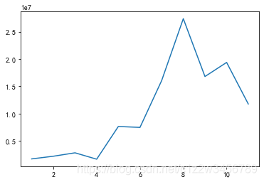
#6.1.2每月的GMV:
#GMV8月之前都基本是处于上升状态,在7月8月的上升更是非常大,8月达到峰值,然后就开始下降了

GMV_month = data.groupby('month').agg(GMV=('amount','sum'))
GMV_month
Out[5]: 
              GMV
month            
1      1729464.93
2      2216672.31
3      2841015.58
4      1674450.68
5      7657332.51
6      7489312.32
7     16048807.99
8     27380899.66
9     16797132.61
10    19376572.75
11    11774974.54

plt.plot(GMV_month.index,GMV_month['GMV'])
plt.show()

 #6.1.3客单价:1240元
#按客户数量

round(data['amount'].sum() / data['user_id'].nunique(),0)
Out[7]: 1240.0

#按订单数量

round(data['amount'].sum() / data['order_id'].nunique(),0)
Out[8]: 296.0

####6.2用户分析
#6.2.1结论先行:
'''
各地区用户最多的是广东(21382),然后是上海(16031)、北京(15928),其他8个城市比较平均(在5400上下)
广东人口基数是全国最高的，而且目前广东的用户仅占广东人口总数的0.017%，最高用户占比是北京：0.0728%，约为广东的4倍，所以在广东投入拉新活动性价比是比较高的
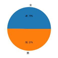
男性和女性用户各占一半
年龄分布也平均，总体上是在16-50岁之间
'''
#转换为日期格式

data['date'] = pd.to_datetime(data['date'])

data.user_id.nunique()
Out[10]: 92755

#6.2.3各地区用户数量

local = data.groupby('local')['user_id'].nunique().reset_index()
local = local.rename(columns={'user_id':'用户数量'})
local = local.sort_values('用户数量').reset_index(drop=True)
local
Out[11]: 
   local   用户数量
0     湖南   5330
1     天津   5337
2     重庆   5342
3     湖北   5355
4     浙江   5370
5     四川   5445
6     海南   5449
7     江苏   5561
8     北京  15928
9     上海  16031
10    广东  21382

plt.figure(figsize=(10,8))
plt.ylabel('用户数量')
plt.title('各地区用户数量')
plt.bar(local['local'],local['用户数量'])
for x,y in enumerate(local['用户数量']):
    plt.text(x,y+200,y,ha='center')
plt.show()

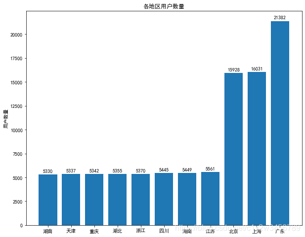
 #广东的用户数量是最多的,然后就是北京和上海,其他八个城市用户比较平均,都是在5400左右。
#6.2.3.1根据2020年的全国人口普查，在网上得到了各省的人口数量数据，分析各省用户的占比，看看哪些省还可以进行用户拉新

population = pd.read_excel(r'F:\Python\合鲸社区\05-某电子产品销售数据分析报告及RFM模型\2020年各省人口数量.xlsx') #网上搜集的
population = population.iloc[:,:2]
population.head()
Out[13]: 
   地区         人口数
0  全国  1411778724
1  广东   126012510
2  山东   101527453
3  河南    99365519
4  江苏    84748016

local = pd.merge(local,population,how='inner',left_on='local',right_on='地区')

local['占比'] = local['用户数量'] / local['人口数']
local = local.sort_values('占比',ascending=False).reset_index(drop=True)
local
Out[15]: 
   local   用户数量  地区        人口数   占比
0     北京  15928  北京   21893095 0.00
1     上海  16031  上海   24870895 0.00
2     海南   5449  海南   10081232 0.00
3     天津   5337  天津   13866009 0.00
4     广东  21382  广东  126012510 0.00
5     重庆   5342  重庆   32054159 0.00
6     湖北   5355  湖北   57752557 0.00
7     浙江   5370  浙江   64567588 0.00
8     湖南   5330  湖南   66444864 0.00
9     江苏   5561  江苏   84748016 0.00
10    四川   5445  四川   83674366 0.00

从上表可以看到,用户数量占比前三是北京、上海、海南，第四是天津,广东排第五,广东的占比仅为第一名北京的五分之一，加上广东的人口数是最多的，所以在广东进行拉新活动的性价比是最高的

#6.2.4用户性别分布

sex =  data.groupby('sex')['user_id'].nunique().reset_index()
sex.rename(columns={'user_id':'用户数量'},inplace=True)
sex
Out[16]: 
  sex   用户数量
0   女  47235
1   男  47628

plt.pie(sex['用户数量'],labels=sex['sex'],autopct='%1.2f%%')
plt.show()

#6.2.5年龄分布

data.age.min()
Out[18]: 16.0

data.age.max()
Out[19]: 50.0

bins = [15,20,25,30,35,40,45,50]
labels = ['(15-20]岁','(20-25]岁','(25-30]岁','(30-35]岁','(35-40]岁','(40-45]岁','(45-50]岁']
data_ = data.copy()
data_['age_bin'] = pd.cut(x=data.age,bins=bins,right=True,labels=labels)
data_
Out[20]: 
                   order_id           product_id  ...  amount   age_bin
0       2294359932054536986  1515966223509089906  ...  324.02  (20-25]岁
1       2294444024058086220  2273948319057183658  ...  155.04  (35-40]岁
2       2294584263154074236  2273948316817424439  ...  217.57  (30-35]岁
3       2295716521449619559  1515966223509261697  ...   39.33  (15-20]岁
4       2295740594749702229  1515966223509104892  ... 5548.04  (20-25]岁
                    ...                  ...  ...     ...       ...
536306  2388440981134693942  1515966223526602848  ...  138.87  (20-25]岁
536307  2388440981134693943  1515966223509089282  ...  418.96  (20-25]岁
536308  2388440981134693944  1515966223509089917  ...   12.48  (15-20]岁
536309  2388440981134693944  2273948184839454837  ...   41.64  (15-20]岁
536310  2388440981134693944  1515966223509127566  ...   53.22  (15-20]岁

[535065 rows x 17 columns]

age = data_.groupby('age_bin')['user_id'].nunique().reset_index()
age.rename(columns={'user_id':'用户数量'},inplace=True)
age
Out[21]: 
    age_bin   用户数量
0  (15-20]岁  13726
1  (20-25]岁  13867
2  (25-30]岁  13831
3  (30-35]岁  13802
4  (35-40]岁  13775
5  (40-45]岁  13969
6  (45-50]岁  13535

plt.figure(figsize=(10,4))
plt.bar(age['age_bin'],age['用户数量'])
plt.show()

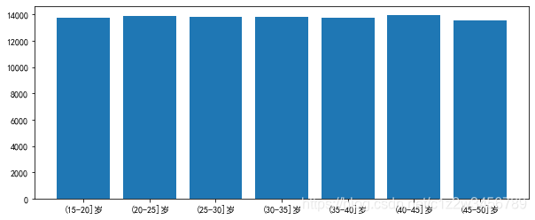
 用户年龄分布较平均,在16-50岁

data_.groupby('age')['user_id'].nunique().reset_index()
Out[23]: 
     age  user_id
0  16.00     2797
1  17.00     2725
2  18.00     2759
3  19.00     2703
4  20.00     2838
5  21.00     2786
6  22.00     2792
7  23.00     2820
8  24.00     2764
9  25.00     2768
10 26.00     2793
11 27.00     2724
12 28.00     2825
13 29.00     2802
14 30.00     2755
15 31.00     2772
16 32.00     2841
17 33.00     2745
18 34.00     2738
19 35.00     2764
20 36.00     2805
21 37.00     2710
22 38.00     2820
23 39.00     2813
24 40.00     2685
25 41.00     2753
26 42.00     2763
27 43.00     2875
28 44.00     2854
29 45.00     2784
30 46.00     2713
31 47.00     2677
32 48.00     2781
33 49.00     2707
34 50.00     2724

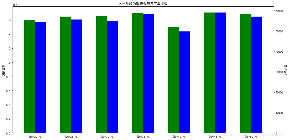
#6.2.6各年龄段的消费金额及下单数量
发现35-40岁的用户,贡献的消费金额与下订单的数量都是最低的,其他年龄段比较平均
age_bin_data = data_.groupby('age_bin').agg(消费金额=('amount','sum'),下单次数=('order_id','nunique'))
age_bin_data
Out[24]: 
                消费金额   下单次数
age_bin                    
(15-20]岁 16007287.18  54302
(20-25]岁 16500743.70  55546
(25-30]岁 16513446.00  54723
(30-35]岁 17004578.70  58275
(35-40]岁 14995577.44  49744
(40-45]岁 17078724.54  59067
(45-50]岁 16886278.32  57085

fig,ax1 = plt.subplots(figsize=(16,8))
xticks = np.arange(len(age_bin_data.index))

ax1.bar(xticks,age_bin_data.消费金额,width=0.3,color='g')
ax1.set_ylabel('消费金额')
ax2 = ax1.twinx()

ax2.bar(xticks+0.3,age_bin_data.下单次数,width=0.3,color='b')
ax2.set_ylabel('下单次数')
plt.title('各年龄段的消费金额及下单次数')

ax1.set_xticks(xticks+0.15)
ax1.set_xticklabels(age_bin_data.index)
plt.show()

#6.2.7男性女性的消费金额及下单数量
#发现男性女性的消费金额与下单次数均比较平均

sex_data = data_.groupby('sex').agg(消费金额=('amount','sum'),下单次数=('order_id','nunique'))
sex_data
Out[26]: 
           消费金额    下单次数
sex                    
女   57108456.57  192394
男   57878179.31  196348

#6.2.8分析购买了0元产品的用户
#从产品的类别可以知道,0元的商品应该是抽奖活动中奖的
#中奖的30个用户中,仅有1个用户没有购买过其他商品,而且这30个用户的客单价高达34832元(总的客单价为1240元)
data[data['price']==0]
Out[27]: 
                   order_id           product_id  ... buy_cnt amount
18846   2323108762694451619  1515966223509132095  ...       1   0.00
39974   2348769908982022577  2309018259719979217  ...       1   0.00
47017   2348779162900103916  2309018259719979217  ...       1   0.00
56572   2348791961667764924  2309018259719979217  ...       1   0.00
61602   2348798941820092785  1515966223509118512  ...       1   0.00
62416   2348799560932918101  2309018259719979217  ...       1   0.00
63934   2348801959043007423  1515966223509117560  ...       1   0.00
64171   2348802240422084738  2309018259719979217  ...       1   0.00
73950   2348816074318807631  2309018259719979217  ...       1   0.00
105538  2353232124972106231  2309018259719979217  ...       1   0.00
118650  2353259718920634989  2309018259719979217  ...       1   0.00
122452  2353267147829937068  2309018259719979217  ...       1   0.00
126484  2353276891760165720  2309018259719979217  ...       1   0.00
138497  2354499489466679644  1515966223509117182  ...       1   0.00
290457  2383131432571633684  2309018260114244280  ...       1   0.00
325835  2388440981134432748  2309018260114244280  ...       1   0.00
340713  2388440981134469495  2309018260114244280  ...       1   0.00
361988  2388440981134532738  2309018260114244281  ...       1   0.00
395362  2388440981134591174  2309018260114244281  ...       1   0.00
407040  2388440981134600026  2309018260114244280  ...       1   0.00
427892  2388440981134615512  2309018260114244280  ...       1   0.00
429370  2388440981134616477  2309018260114244280  ...       1   0.00
430578  2388440981134617284  2309018260114244280  ...       1   0.00
434932  2388440981134620423  2309018259719979217  ...       1   0.00
435548  2388440981134620837  2309018260114244281  ...       1   0.00
444242  2388440981134627558  2309018260114244280  ...       1   0.00
445869  2388440981134628677  2309018259719979217  ...       1   0.00
475017  2388440981134649580  2309018260114244281  ...       1   0.00
494181  2388440981134663702  2309018260114244281  ...       1   0.00
514493  2388440981134678374  2309018260114244280  ...       1   0.00

[30 rows x 16 columns]

#提取该批用户出来
user_0 = data[data['price']==0]['user_id'].reset_index(drop=True)
user_0
Out[28]: 
0     1515915625468531712
1     1515915625484619520
2     1515915625484629760
3     1515915625446572032
4     1515915625484641280
5     1515915625484627200
6     1515915625484652288
7     1515915625484648960
8     1515915625446041088
9     1515915625446041088
10    1515915625512678912
11    1515915625486717696
12    1515915625479406336
13    1515915625449238016
14    1515915625498273536
15    1515915625498244096
16    1515915625498229248
17    1515915625505436160
18    1515915625512202240
19    1515915625512377088
20    1515915625512762368
21    1515915625512763136
22    1515915625512763904
23    1515915625512817664
24    1515915625512118784
25    1515915625498201088
26    1515915625513058048
27    1515915625467158528
28    1515915625514162432
29    1515915625514596864
Name: user_id, dtype: object

user_0.shape
Out[29]: (30,)

#30个中奖的用户中,只有一个用户没有产生消费

user_0[~user_0.isin(data[data['price']>0]['user_id'])]
Out[30]: 
0    1515915625468531712
Name: user_id, dtype: object

data_user_0 = pd.merge(data,user_0,on='user_id')

data_user_0_amount = data_user_0.groupby('user_id').agg(消费金额=('amount','sum')).sort_values('消费金额',ascending=False)
data_user_0_amount
Out[32]: 
                         消费金额
user_id                      
1515915625512377088 149967.06
1515915625512763904 109908.68
1515915625512763136  77031.07
1515915625514596864  76281.00
1515915625512817664  76046.94
1515915625512118784  65778.93
1515915625513058048  58286.07
1515915625512202240  52518.51
1515915625514162432  48217.85
1515915625484627200  46833.03
1515915625484652288  46558.67
1515915625484648960  42259.39
1515915625512762368  37710.57
1515915625484641280  26495.51
1515915625484629760  26273.05
1515915625484619520  25002.66
1515915625479406336  15143.98
1515915625486717696  14081.96
1515915625446572032  10451.64
1515915625498273536   8553.32
1515915625446041088   7726.76
1515915625512678912   6487.89
1515915625498201088   6020.53
1515915625498244096   3291.36
1515915625505436160   2908.19
1515915625498229248   2317.66
1515915625467158528   1925.24
1515915625449238016    893.42
1515915625468531712      0.00

#该批用户的客单价为34832元

data_user_0_amount['消费金额'].sum() / 30
Out[33]: 34832.36466666667

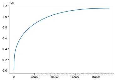
#6.2.9二八定律-找出累计贡献销售额80%的那批用户
#前27%的用户贡献了80%的销售收入,这批用户要做好跟进,一定要留住这批贡献大的客户

user_28 = data.groupby('user_id').agg(消费金额=('amount','sum')).sort_values('消费金额',ascending=False).reset_index()
user_28['累计销售额'] = user_28['消费金额'].cumsum()
user_28
Out[34]: 
                   user_id      消费金额        累计销售额
0      1515915625512422912 160604.07    160604.07
1      1515915625513695488 158277.37    318881.44
2      1515915625512377088 149967.06    468848.50
3      1515915625513577472 135672.84    604521.34
4      1515915625514597888 133945.88    738467.22
                   ...       ...          ...
92750  1515915625511079936      0.02 114986635.82
92751  1515915625450548736      0.02 114986635.84
92752  1515915625506653440      0.02 114986635.86
92753  1515915625451367168      0.02 114986635.88
92754  1515915625468531712      0.00 114986635.88

[92755 rows x 3 columns]

#前27%的用户贡献了80%的销售收入
 

p = user_28['消费金额'].cumsum()/user_28['消费金额'].sum()  # 创建累计占比，Series
key = p[p>0.8].index[0] 
key
Out[35]: 25408

key / user_28.shape[0]
Out[36]: 0.2739259339119185

plt.plot(user_28.index,user_28['累计销售额'])
plt.show()

         

#6.2.10客户消费金额的分位数
#用户平均消费金额大于75%分位数,即存在着高消费的客户

data.groupby('user_id').agg(消费金额=('amount','sum')).describe(percentiles=(0.01,0.1,0.25,0.75,0.9,0.99)).T
Out[38]: 
        count    mean     std  min  ...     75%     90%      99%       max
消费金额 92755.00 1239.68 4129.72 0.00  ... 1141.17 2402.53 12744.87 160604.07

[1 rows x 12 columns]

#6.2.11客户消费周期
#消费了两次及以上的客户有50%的消费周期为7天内,用户的消费周期还是比较短的。75%为26天内，消费周期适中
purchase_day = data[data['amount']>0].sort_values('date').groupby('user_id').apply(lambda x: x['date'] - x['date'].shift()).dt.days
purchase_day
Out[39]: 
user_id                    
1515915625439951872  90907      nan
1515915625440038400  357719     nan
                     461674   36.00
1515915625440051712  451057     nan
                     451029    0.00

1515915625514888704  536285     nan
                     536306    0.00
                     536275    0.00
1515915625514891008  536300     nan
1515915625514891264  536307     nan
Name: date, Length: 535035, dtype: float64

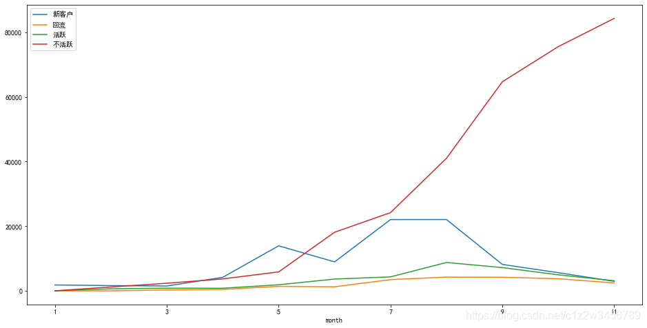
#6.2.12每月新客户、不活跃客户、回流客户、活跃客户的情况

purchase_day[purchase_day>0].describe(percentiles=[0.01,0.1,0.25,0.75,0.9,0.99])
Out[40]: 
count   139989.00
mean        21.06
std         31.44
min          1.00
1%           1.00
10%          1.00
25%          2.00
50%          7.00
75%         26.00
90%         63.00
99%        146.00
max        299.00
Name: date, dtype: float64

pivoted_amount =data[data['amount']>0].pivot_table(index='user_id'
                                             ,columns='month'
                                             ,values='buy_cnt'
                                             ,aggfunc='sum').fillna(0)
columns_month = pivoted_amount.columns.astype('str')  #一定要把列名格式变为str不然后面就会报错
pivoted_amount.columns = columns_month
pivoted_purchase = pivoted_amount.applymap(lambda x:1 if x>0 else 0)

def active_status(data):
    status =[]
    for i in range(11):
        #若本月没有消费
        if data[i] ==0:
            if len(status)>0:  #如果不是第一个月,
                if status[i-1]=='未注册': #如果上个月已经是未注册,那么本月也是未注册
                    status.append('未注册') 
                else:  #如果上月已注册,则本月为不活跃
                    status.append('不活跃')
            else:  #如果是第一个月
                status.append('未注册') #则未注册
        #若本月消费
        else:
            if len(status)==0: #如果是第一个月,则为新注册用户
                status.append('新客户')
            else:  #如果不是第一个月
                if status[i-1]=='不活跃':  #如果上月为不活跃,那么本月为回流
                    status.append('回流')
                elif status[i-1]=='未注册':  #如果上月为未注册,那么本月为新注册
                    status.append('新客户')
                else:  #如果上月为活跃,本月也为活跃
                    status.append('活跃')
    return pd.Series(status,index=columns_month)

pivoted_purchase_status = pivoted_purchase.apply(lambda x:active_status(x),axis=1)
pivoted_purchase_status.head()
Out[43]: 
month                  1    2    3    4    5    6    7    8    9   10   11
user_id                                                                   
1515915625439951872  未注册  未注册  未注册  未注册  未注册  未注册  新客户  不活跃  不活跃  不活跃  不活跃
1515915625440038400  未注册  未注册  未注册  未注册  未注册  未注册  未注册  未注册  新客户   活跃  不活跃
1515915625440051712  未注册  未注册  未注册  未注册  未注册  未注册  未注册  未注册  未注册  新客户   活跃
1515915625440099840  未注册  未注册  未注册  未注册  新客户   活跃   活跃  不活跃   回流   活跃   活跃
1515915625440121600  未注册  未注册  未注册  未注册  新客户  不活跃   回流  不活跃  不活跃  不活跃  不活跃

purchase_cnt = pivoted_purchase_status.apply(lambda x:x.value_counts())
#去除未注册的数据行
purchase_cnt = purchase_cnt[purchase_cnt.index != '未注册']
purchase_cnt = purchase_cnt.fillna(0)
#排序 可排可不排
purchase_cnt = purchase_cnt.loc[['新客户','回流','活跃','不活跃'],:]
purchase_cnt
Out[44]: 
month       1       2     3     4      5  ...      7      8      9     10       11
新客户   1813.00 1613.00  1491  4177  13914  ...  22036  22052   8163   5607  2938.00
回流       0.00    0.00   261   432   1377  ...   3462   4244   4199   3740  2444.00
活跃       0.00  623.00   819   800   1865  ...   4309   8765   7182   4941  3116.00
不活跃      0.00 1190.00  2346  3685   5852  ...  24187  40985  64665  75528 84256.00

[4 rows x 11 columns]

purchase_cnt.T.plot(figsize=(16,8))
Out[45]: <matplotlib.axes._subplots.AxesSubplot at 0x218e29bc708>